Introduction
Pseudonoise sequences are bit streams used in communications engineering for spread spectrum communications, radio distance measurements, and analyzing concert hall acoustics during live performances.
This is due to their sharply peaked autocorrelation properties. We'll show how their properties can be derived directly from Galois field arithmetic. We'll generalize to mod p arithmetic, leaving the binary PN sequences as a special case when p=2.
We'll conclude by showing how to build a mechanical autocorrelator as a teaching tool which dramatically demonstrates their properties. This is a new and unique design for which there exists no prior art to the best of my knowledge.
Prerequisites: Knowledge of Galois (finite) field theory.
Finite Field Review
Notation: Let the unique Galois field with $p^n$ elements be denoted $GF( p^n )$
Let a primitive monic polynomial which generates it be $f(x) = x^n + f_{n-1}x^{n-1}+ \ldots + f_1 x + f_0$
The exponential and polynomial forms of the field elements are $$\alpha^{-\infty} = 0$$ $$\alpha^0 = 1$$ $$\alpha = x$$ $$\ldots$$ $$\alpha^k = x^k (mod \: f(x),p)$$ $$\ldots$$ $$\alpha^{p^n-2} = x^{p^n-2} (mod \: f(x),p)$$
Example: The field with 16 elements, $GF( 2^4 )$ is generated by the primitive polynomial, $f(x) = x^4 + x + 1$ which has as elements, $$\alpha^{-\infty} = 0$$ $$\alpha^0 = 1$$ $$\alpha^1 = x$$ $$\ldots$$ $$\alpha^{13} = x^3+x^2+1$$ $$\alpha^{14}=x^3+1$$ $$\alpha^{15}=1$$
Pseudonoise Sequences
Definition. The pseudonoise (PN) sequence of length $p^n-1$ is the sequence $\left\{ b_k \right\}_{k=0}^{p^n-2}$ where $b_k = (-1)^{a_k}$ and $a_k$ = constant coefficient of the polynomial representation of field element $\alpha^k$ When the Galois field elements are written out as a list of polynomial coefficients, the PN sequence is the last column.
Example: reading off the constant coefficient of the polynomials in our example field we get $${1,0,0,0,1,0,0,1,1,0,1,0,1,1,1}$$ which generates the length 15 sequence $${-1,+1,+1,+1,-1,+1,+1,-1,-1,+1,-1,+1,-1,-1,-1}$$
Difference Equation
We don't need to generate the field and do time consuming finite field arithmetic to find a PN sequence, but can use a recursive method instead.
Note that $f(x) \equiv 0 (mod \: f(x),p)$ and so $x^k f(x) \equiv 0 (mod \: f(x),p) \text{ for } 0 \le k \le p^n-2$
Expanding out we get $$x^{n+k} + f_{n-1} x^{n+k-1} + \ldots + f_1 x^{k+1} + f_0 x^k \equiv 0 (mod \: f(x),p)$$ Now applying the mod operation throughout, $$\alpha^{n+k} + f_{n-1} \alpha^{n+k-1} + \ldots + f_1 \alpha^{k+1} + f_0 \alpha^k \equiv 0$$ Take the constant coefficient of each polynomial term, $$a_{n+k} + f_{n-1} a_{n+k-1} + \ldots + f_1 a_{k+1} + f_0 a_k \equiv 0 (mod \: p)$$ And rearrange to get the difference equation, $$a_{n+k} = -(f_{n-1} a_{n+k-1} + \ldots + f_1 a_{k+1} + f_0 a_k)(mod \: p)$$ for $0 \le k \le p^n-2$
with initial conditions $$a_0 = ( \text{ const coeff of polynomial for } \alpha^0 ) = 1$$ $$a_1 = ( \text{ const coeff of polynomial for } \alpha^1 ) = 1$$ $$\ldots$$ $$a_n = ( \text{ const coeff of polynomial for } \alpha^{n-1} ) = 1$$
That is, the all zeros except for the first coefficient.
Example: $$a_0 = 1, \: a_1 = a_2 = a_3 = 0$$ are the initial conditions and the difference equation is $$a_{k+4} = -(a_{k+1} + a_k) = (a_{k+1} + a_k) (mod \: 2)$$ which generates the same PN sequence as before (Note that we can omit the -1 since -1 = 1 (mod 2)). $$a_4 = a_1 + a_0 = 1 (mod \: 2)$$ $$a_5 = a_2 + a_1 = 0 (mod \: 2)$$ We continue shifting until we come back to the initial state at $k = 2^4-1=15$.
Hardware Implementation
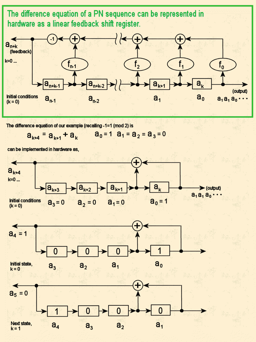
| k | ak+4(feedback) | ak+3 | ak+2 | ak+1 | ak(output) |
|---|---|---|---|---|---|
| 0 | 1 | 0 | 0 | 0 | 1 |
| 1 | 0 | 1 | 0 | 0 | 0 |
| 2 | 0 | 0 | 1 | 0 | 0 |
| 3 | 1 | 0 | 0 | 1 | 0 |
| 4 | 1 | 1 | 0 | 0 | 1 |
| 5 | 0 | 1 | 1 | 0 | 0 |
| ... | ... | ... | ... | ... | ... |
| 14 | 0 | 0 | 0 | 1 | 1 |
| 15 | 1 | 0 | 0 | 0 | 1 (same as k=0) |
Software Implementation
In the C language, we can emulate the hardware bit operations with bit shifting and masking. Here is sample C code which computes values of a binary PN sequence. Source code Version 1.0 is distributed under the terms of the GNU General Public License. You will need to download each of the files below.
The program output is,
pn 1 = 1, pn 2 = 0, pn 3 = 0, pn 4 = 0, pn 5 = 1, pn 6 = 0
pn 7 = 0, pn 8 = 1, pn 9 = 1, pn 10 = 0, pn 11 = 1, pn 12 = 0
pn 13 = 1, pn 14 = 1, pn 15 = 1
Circular Autocorrelation
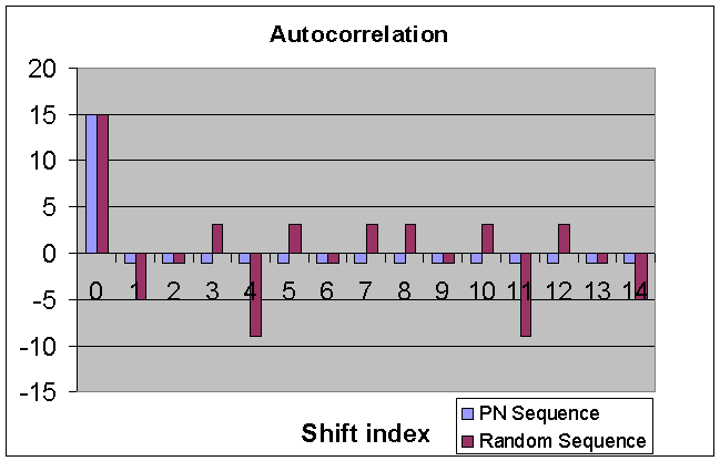
The circular autocorrelation of the PN sequence $\left\{ b_k \right\}_{k=0}^{p^n-2}$ is defined to be $c_j = \sum_{k=0}^{p^n-2} b_k b_{k+j} \text{ for } 0 \le j \le p^n-1$ where indices are taken modulo $p^n-1$ We will show that in the binary case p=2, the autocorrelation has a sharp peak at j=0 and is flat elsewhere.
Example. Our sample sequence has autocorrelation, $$C_0 = 15, \: c_1 = \ldots = c_{14} = -1$$ We get $$c_0 = \{-1,+1,+1,+1,-1,+1,+1,-1,-1,+1,-1,-1,-1 \} \ast $$ $$\{ -1,+1,+1,+1,-1,+1,+1,-1,-1,+1,-1,+1,-1,-1 \} = 15$$ $$c_1 = \{-1,+1,+1,+1,-1,+1,+1,-1,-1,+1,-1,+1,-1,-1,-1 \} \ast $$ $$\{ +1,+1,+1,-1,+1,+1,+1,+1,-1,-1,+1,-1,+1,-1,-1,-1,-1 \} = -1$$ $$\ldots$$ The autocorrelation is very sharply peaked: $$\{ 15, -1, -1, -1, -1, -1, -1, -1, -1, -1, -1, -1, -1, -1, -1 \}$$ I tossed a penny 15 times to get a random sequence, $$\{ +1, -1, -1, -1, +1, +1, -1, +1, -1, -1, +1, -1, +1, +1, -1 \}$$ and the autocorrelation was much less sharply peaked: $$\{ 15, -5, -1, +3, -9, +3, -1, +3, +3, -1, +3, -9, +3, -1, -5 \}$$
Theorem. The circular autocorrelation of the PN sequence, $$c_j = \sum_{k=0}^{p^n-2} b_k b_{k+j} \text{ for } 0 \le j \le p^n-1$$ is $$ c_j = \begin{cases} p^{n-1} \quad \quad \text{ any p } \quad \quad j = 0 \\ p^n-1 \quad \text{ odd p } \quad \quad 1 \le j \le p^{n-1} \\ 0 \quad \quad \quad p = 2 \quad \quad 1 \le j \le p^{n-1} \\ \end{cases} $$
Proof.
Case j=0:
$c_0 = \sum_{k=0}^{p^n-2} b_k^2 = \sum_{k=0}^{p^n-2} 1 = p^n-1$
Case $1 \le j \le p^n-1$
$c_j = \sum_{k=0}^{p^n-2} b_k b_{k+j} = \sum_{k=0}^{p^n-2} (-1)^{a_k + a_{k+j}}$ where indices are taken modulo $p^n-1$ Now we digress to note that since $\alpha$ is a primitive element of the field we can write $1 + \alpha^j = \alpha^{Z(j)} \text{ for } -\infty \le j, Z(j) \le p^n-2$ where $Z(j)$ is called the Zech's logarithm of $j$. $Z(j) \neq -\infty$ since the unique inverse of 1 is p-1, which will not happen. $$\alpha^k + \alpha^{k+j} = \alpha^k \alpha^{Z(j)} = \alpha^{k+Z(j)}$$ rewriting into polynomial form, taking mod f(x) and p, and looking at the constant term gives, $$a_k + a_{k+j} = a_{k+Z(j)}$$ Then $$c_j = \sum_{k=0}^{p^n-2} (-1)^{a_{k+Z(j)}} =$$ $$ \sum_{k=0}^{p^n-2} b_{k+Z(j)} = \sum_{k=0}^{p^n-2} b_k$$ where the last step follows because the indices are merely shifted modulo $p^n-1$ Now consider the sum for even p and odd p cases. $\blacksquare$
| Field Elements | bk | Partial Sum |
|---|---|---|
| 0 | 1 | 1 |
| 1 | -1 | 0 |
| 2 | 1 | 1 |
| 3 | -1 | 0 |
| 4 | 1 | 1 |
| x+0 | 1 | 1 |
| x+1 | -1 | 0 |
| x+2 | 1 | 1 |
| x+3 | -1 | 0 |
| x+4 | 1 | 1 |
| ... | ... | ... |
| 3x2+0 | 1 | 1 |
| 3x2+1 | -1 | 0 |
| 3x2+2 | 1 | 1 |
| 3x2+3 | -1 | 0 |
| 3x2+4 | 1 | 1 |
| Field Elements | bk | Partial Sum |
|---|---|---|
| 0 | 1 | 1 |
| 1 | -1 | 0 |
| x+0 | 1 | 1 |
| x+1 | -1 | 0 |
| x2+0 | 1 | 1 |
| x2+1 | -1 | 0 |
| ... | ... | ... |
| x3+x2+x+0 | 1 | 1 |
| x3+x2+x+1 | -1 | 0 |
Now each group of odd p constant coefficients has an extra unpaired 1. Number of groups = (total number of field elements) / p = $\frac{p^n}{p} = p^{n-1}$
Mechanical Autocorrelator
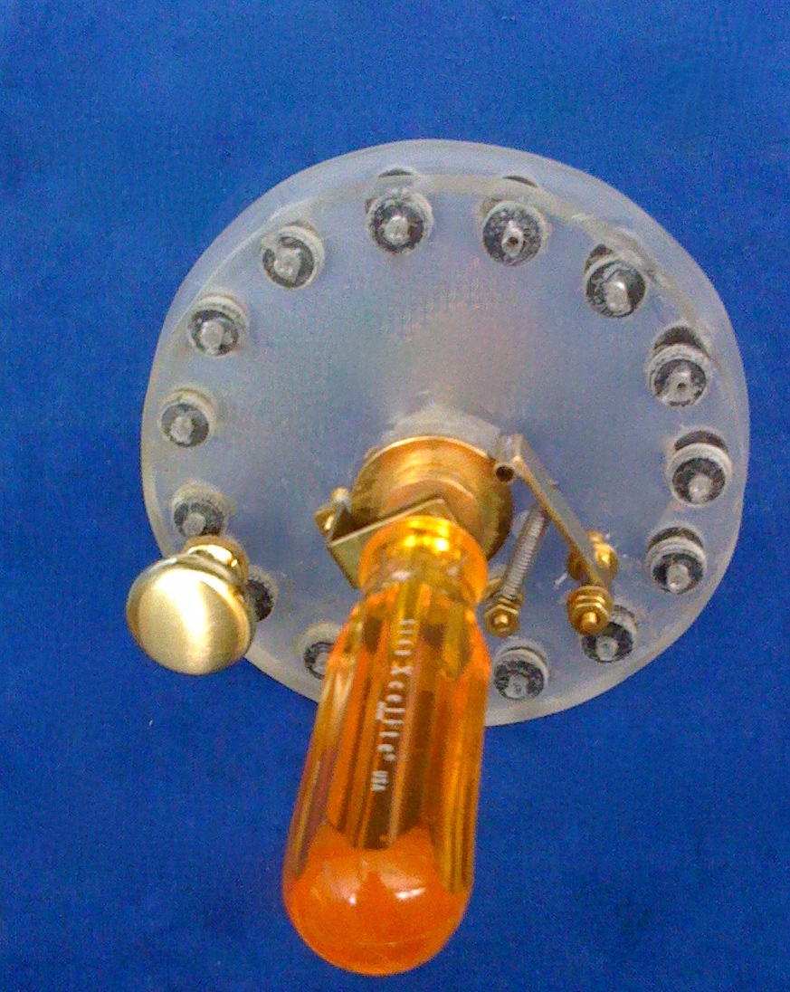
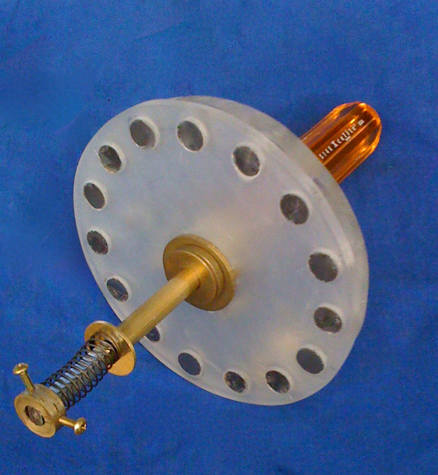
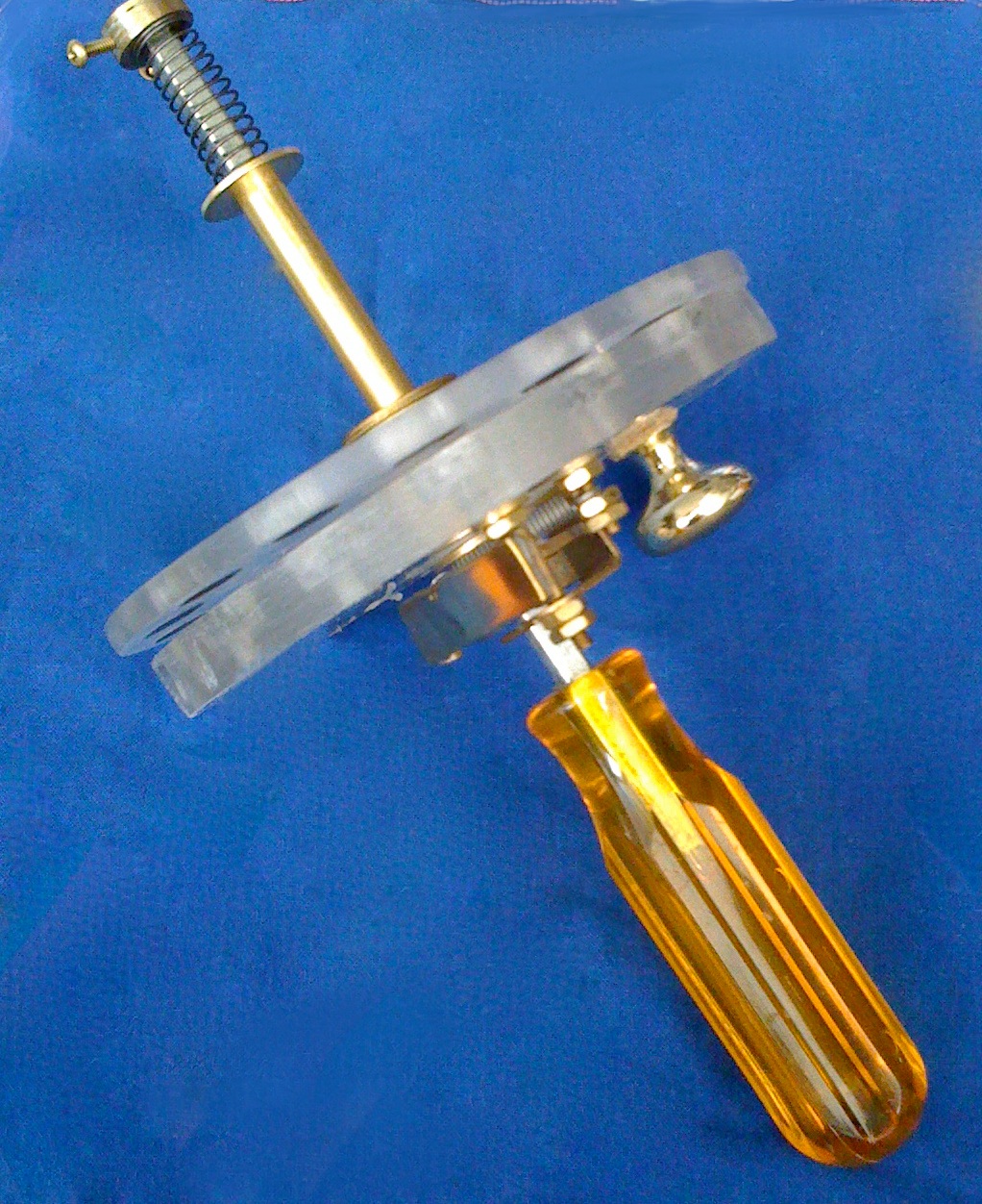
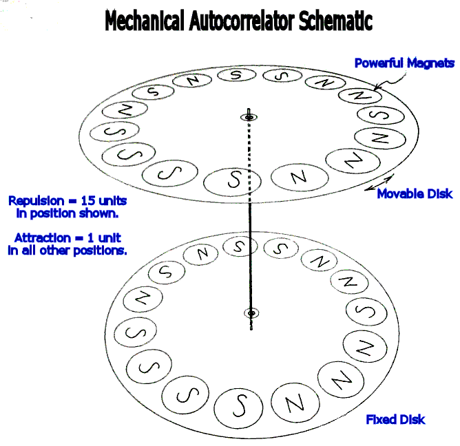
To illustrate the autocorrelation properties of the PN sequence, I've designed a mechanical autocorrelator.
The device is made of two plastic disks which rotate on a common axis. Each disk has $2^m-1$ magnets equally spaced along its rim. A ratchet and pawl mechanism contrains the magnets to hold positions in which they line up facing each other when the disks are rotated. When rotated, the disks attract each other in all positions (autocorrelation minima) except one --- in that position (autocorrelation maximum), they repel very strongly.
The figure shows a mechanical autocorrelator based on the binary PN sequence of our examples of length 15.
Let's demonstrate the connection between the autocorrelation formula just proved and our analog computer.
Theorem. When similar magnets line up, the disks repel with a force of $2^m-1$ magnet pairs, corresponding to the autocorrelation peak at j=0. In all other positions, the disks attract with the force of 1 magnet pair, corresponding to the autocorrelation minima of -1.
Proof. We set up a direct correspondence between the equations and the mechanism. As Sherlock Holmes would say, "The parallel is exact". $\blacksquare$
| Correspondence | |
| PN Equation | Mechanism |
| bk=+1 | North pole of magnet facing up |
| bkbk+j=+1 | Repulsion of magnets k and k+j |
| bkbk+j=-1 | Attraction of magnets k and k+j |
| cj | Sum of forces of all 2n-1 magnet pairs in offset position j |
References
- M. R. Schoeder, NUMBER THEORY IN SCIENCE AND COMMUNICATION, 2nd enlarged edition, Springer-Verlag, 1986.